Research Dispatch 001Open journal record

A simpler rule beat the hierarchy on GPT-2. Here’s what that means.

I built a sophisticated hierarchy to compress neural networks without erasing rare-domain behavior. It worked perfectly in a controlled setting. On GPT-2, a much simpler robust baseline did better at aggressive compression—and that became the real result.

Analysis byKenju Tomita

PublishedAugust 9, 2026

Reading time15 minutes

Research record Read the peer-reviewed article, version history, and source files Ephemerent Research · ER-2026-0001

Three calibration environments

01 · Common prose frequent 02 · Dialogue regular 03 · Code rare

Average selectionKeeps what matters most oftenRare direction can disappear before repair

Robust capacityKeeps what matters anywhereRare direction travels into the smaller layer

Figure 1 · The selection problem. Average calibration rewards frequency. Robust selection asks whether a unit is important in any named environment.Editorial illustration · Ephemerent News

The shortest version: the paper’s robust principle survived contact with GPT-2, but its most elaborate machinery did not earn the win. That is not a failed story. It is a more useful one.

Neural network compression tries to make a model smaller by removing computation it appears not to need. The danger is that “not needed” is usually measured on a calibration sample—and a calibration sample can be very good at representing what is common while barely showing what is rare.

The intuition

The rare musician.

Imagine compressing an orchestra after listening to rehearsals. One musician plays constantly. Another enters only once, during a quiet coda—but without that note, the ending collapses.

If you rank musicians by their average sound across rehearsal, the rare player looks expendable. That judgment is locally reasonable and globally wrong. The sample has confused infrequency with redundancy.

Calibration scoreContribution over time

Commonfrequent

Dialogueregular

Coderare · unique

The rare line is short. Its direction is still irreplaceable.

DR-FSP starts from this concern: a unit that looks redundant on common inputs may carry a computational direction that a rare environment relies on. Its central proposal is to judge importance across named environments, not only in the mixture average.

There is one extra fairness step. Prose, dialogue, and code can naturally produce outputs at different scales, so the paper measures each environment’s reconstruction error relative to that environment’s own original output. In plain language: what fraction of this room’s behavior did compression fail to reproduce?

How robust risk works

Three rooms. Two ways to grade the repair.

Common prose70% of illustrative mixture

R = 0.04

Dialogue25% of illustrative mixture

R = 0.08

Code5% of illustrative mixture

R = 0.42

Prevalence-weighted score 0.07

The frequent rooms dominate the mixture, so a serious code failure can look small in the overall grade.

Illustrative risk units, not measured paper results. A risk of 0 is a perfect reconstruction; a risk around 1 is roughly as much error as replacing the layer contribution with zero. Worst-environment optimization follows the largest normalized error instead of letting prevalence hide it.

The mechanism

What a neuron actually contributes.

A hidden unit has two parts to its job. First, it fires: it recognizes something in the current input. Then it writes: it pushes a direction into the next part of the network.

Looking at only one half can mislead. A unit can activate loudly but write almost nothing useful. Another can fire rarely yet write a direction no surviving unit can reproduce.

01What fires

The inputs that make the unit respond.

02What it writes

The direction it adds to the layer output.

03What survives

The functional direction available after compression.

The paper represents a unit by both its activation pattern and its outgoing write. Compression should preserve the product, not merely the loudest half.

The multiplication is easier to picture than it looks. Take one vertical tape showing how strongly the neuron fired on each example. Multiply it by one horizontal arrow showing where the neuron writes. The result is a sheet: the same write direction repeated for every example, louder or quieter according to the activation tape.

The rank-one operator

One neuron leaves a sheet of evidence.

Stack one contribution sheet for each environment and the unit’s job becomes visible across prose, dialogue, and code.

a_e,iactivation tapev_iwrite directionF_e,icontribution sheet

Selected sheetCommon prose

Frequent activation makes this sheet easy to see in an average calibration sample.

activation over examples outgoing write direction environments

COMMON PROSE

DIALOGUE

CODE · RARE SPIKE

The stack is a visual metaphor, not an extra learned 3D tensor. Formally, each environment contributes one two-dimensional activation-by-write sheet. DR-FSP compares those functional sheets rather than treating a neuron as a single weight magnitude.

The distinction

Choosing is not the same as repairing.

Most compression pipelines contain two decisions that are easy to blur together. Selection chooses which neurons remain. Refitting adjusts the outgoing weights of those survivors so they reproduce the old layer as closely as possible.

Refitting can repair coefficients. It cannot generally invent an activation direction that selection already deleted. Once the rare musician has left the building, turning up the remaining microphones does not recreate the missing note.

01Selectiondefines →
02Available basisconstrains →
03Refit ceilingsets →
04Worst-case riskobserved

SelectionWhich activation basis survives?

Same robust refitDamage reducedMissing direction stays missing

Same robust refitLowest worst-case riskThe needed basis is still present

Selected path

Robust refitting helps the fragile subset, but it cannot synthesize the activation direction that average-weighted selection removed.

Selection changes the available basis. Refitting changes only how the surviving basis is combined. Select either path to follow the consequence.

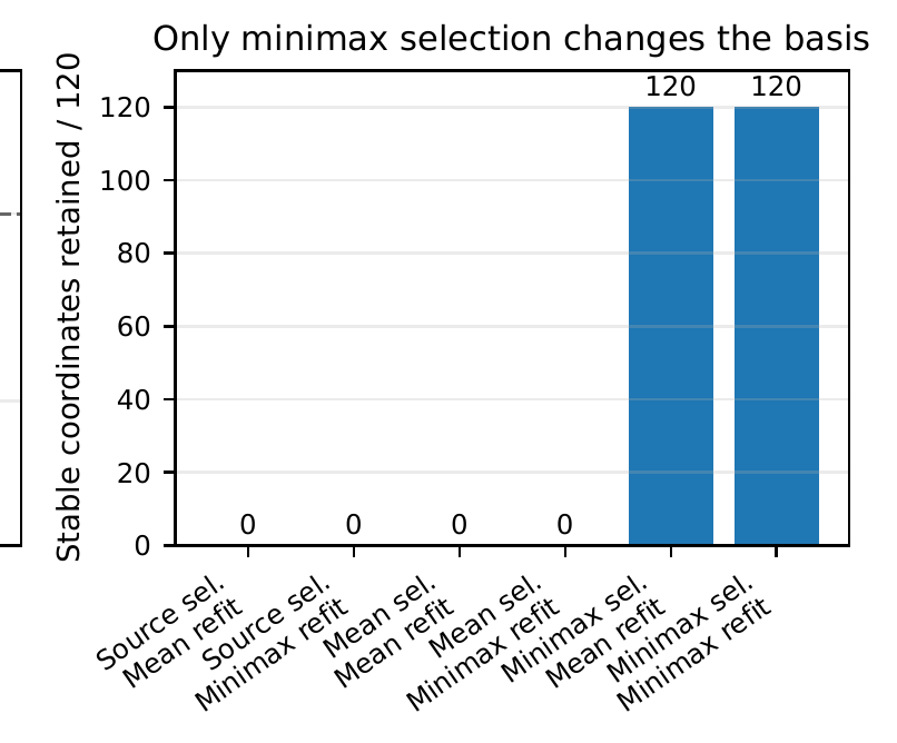
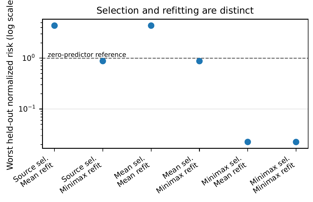
The first controlled experiment made that separation unusually clean. Across 20 seeds, there were six coordinate decisions per seed—120 opportunities to retain the stable direction. Source-only and prevalence-weighted selection kept it 0 out of 120 times. Worst-environment selection kept it 120 out of 120 times and matched an exact search over 729 candidate subsets.

Paper figure · rare environments

Read the right panel first.

Two paper charts showing held-out risk for selection and refitting combinations, and stable coordinates retained out of 120. — **What to notice:** only minimax selection changes which basis survives. A minimax refit lowers the damage of a bad selection, but the right panel remains at zero until the selector itself becomes worst-environment aware.Source DR-FSP manuscript, corrected v3
20 seeds · 120 coordinate decisions

Held-out risk for six combinations of source, average, and minimax selection and refitting. — **What to notice:** only minimax selection changes which basis survives. A minimax refit lowers the damage of a bad selection, but the right panel remains at zero until the selector itself becomes worst-environment aware.Source DR-FSP manuscript, corrected v3
20 seeds · 120 coordinate decisions

The clean win

Where the hierarchy worked.

The more ambitious part of DR-FSP builds a family tree of neurons. Units are grouped by compact functional fingerprints that combine when they fire with what they write. Cut the tree at a target width, keep one representative from each group, then refit globally.

In a controlled overcomplete layer, that structure was exactly the right tool. The synthetic layer contained 100 units but only 50 dominant functional families, mixed with clones, near-clones, distractors, and low-energy directions. The task was to reduce the layer from width 100 to width 50.

Comparing every full contribution sheet would be expensive, so DR-FSP first makes a compact functional fingerprint—more like a contact print than a biography. If two fingerprints preserve the same activation-and-write geometry across environments, the hierarchy can place those units in one family.

Subset projection

Compress the copies, keep the vocabulary.

Before100 unitscopies · near-copies · distractors

After selection50 representativesone dominant family per slot

Then refit

The representatives adjust how strongly they write. They do not have to impersonate a family that selection erased.

Schematic view: five families stand in for the planted fifty. The actual 100→50 experiment included clones, near-clones, distractors, and low-energy directions. The 5% energy floor prevented trivial low-energy units from occupying a family slot.

The aim is not simply to keep the fifty biggest neurons. It is to preserve fifty distinct pieces of functional vocabulary, then let the global refit redistribute responsibility among the survivors.

Hierarchy + energy floor50 / 50

dominant families recovered

Activation-only ranking31.92 / 50

families recovered on average

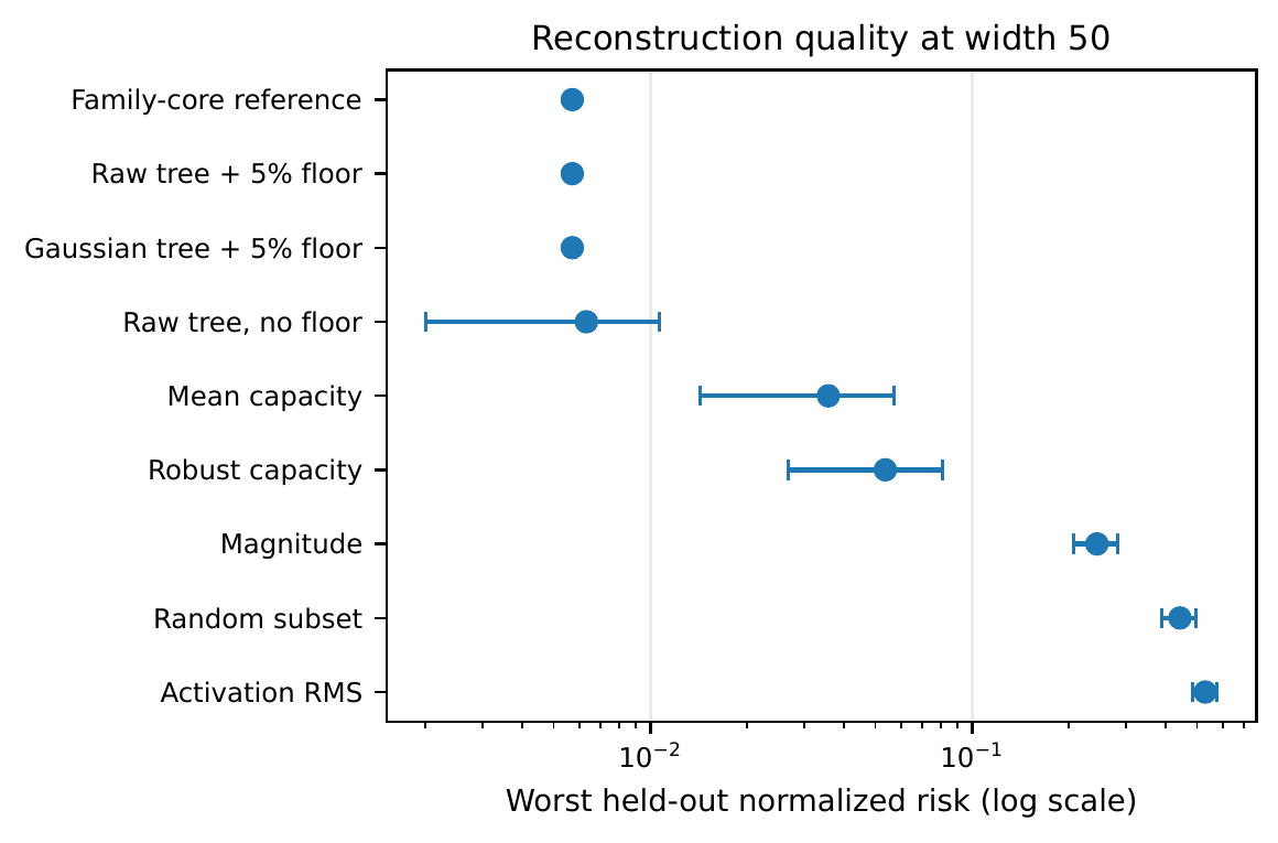
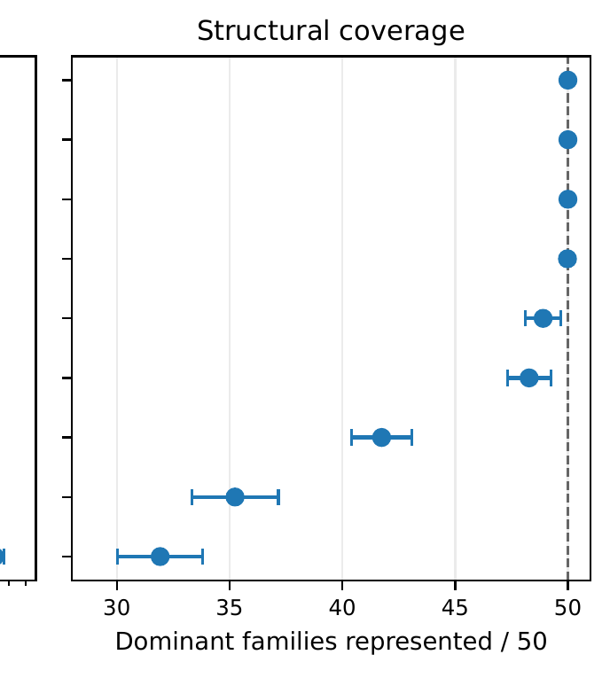
Across 50 random seeds, the raw hierarchy with a declared 5% energy floor recovered all 50 families every time. Magnitude recovered about 41.74; random selection 35.24; activation strength alone 31.92.

Paper figure · controlled compression

Lower risk is left; full family coverage is right.

Two charts comparing reconstruction risk and structural family coverage for controlled width-50 compression methods. — **What to notice:** the three hierarchy/reference rows land at full 50-family coverage. Simpler scalar scores lose families even though every method receives the same robust refit afterward.Source DR-FSP manuscript, corrected v3
100 → 50 units · 50 seeds

Reconstruction quality at width 50 for the hierarchy, capacity scores, magnitude, random selection, and activation strength. — **What to notice:** the three hierarchy/reference rows land at full 50-family coverage. Simpler scalar scores lose families even though every method receives the same robust refit afterward.Source DR-FSP manuscript, corrected v3
100 → 50 units · 50 seeds

The reversal

The GPT-2 surprise.

Then came the harder test: GPT-2 Small. The study compressed one MLP layer at a time—layers 2, 5, and 8—using prose, dialogue, and code as separate environments. It repeated the test across three corpus offsets and three width-reduction levels, producing nine layer-split trials per ratio.

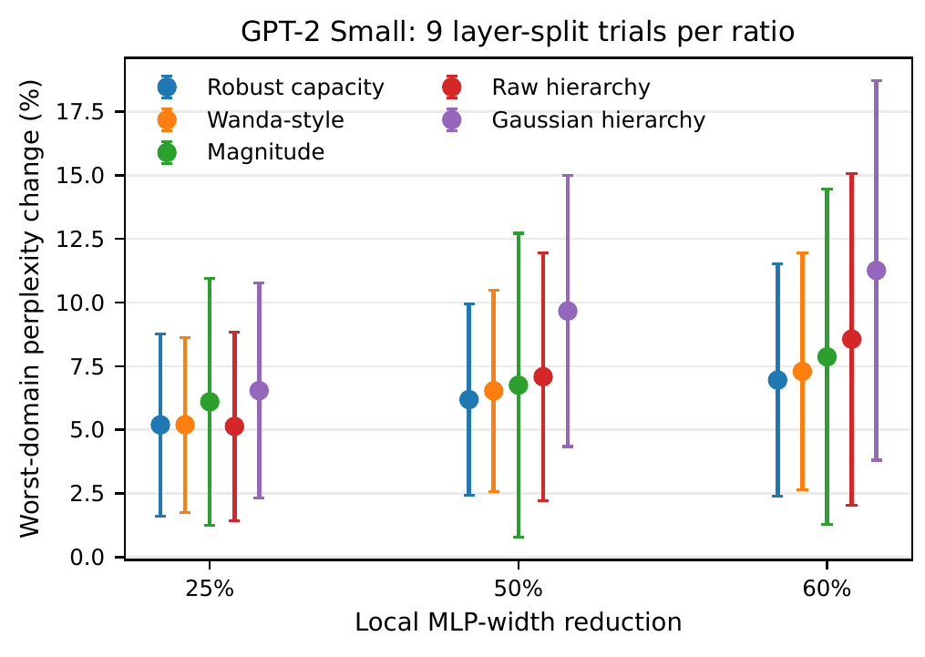
The result did not reward complexity. At a mild 25% local width reduction, raw hierarchy and robust capacity were effectively tied: 5.13% versus 5.19% worst-domain perplexity increase. At 50% and 60% reduction, robust capacity was better: 6.19% vs. 7.09%, then 6.95% vs. 8.56%. Lower is better.

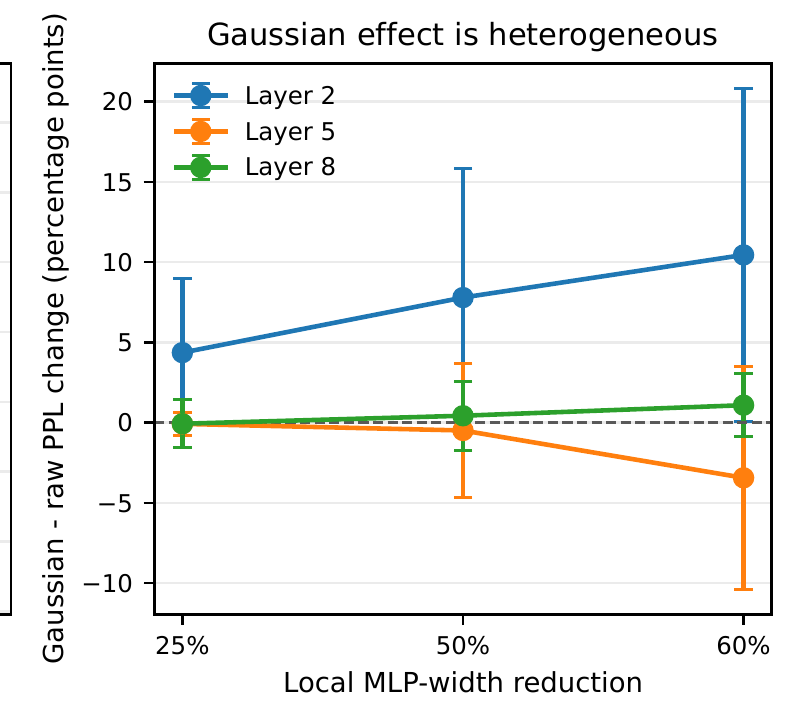
The optional Gaussian refinement did worse still: 6.54%, 9.66%, and 11.26% across the three reductions. A technique intended to stabilize the hierarchy in noisy data appears to have distorted angles that mattered for the natural model.

Paper figure · repeated GPT-2 diagnostic

Lower is better. Error bars show trial variability.

Charts comparing worst-domain perplexity change for five GPT-2 compression selectors at 25, 50, and 60 percent local width reduction. — **What to notice:** blue robust capacity stays lowest at the two aggressive settings. Purple Gaussian hierarchy rises sharply, especially in layer 2. The wide error bars are why this is a diagnostic, not a definitive ranking.Source DR-FSP manuscript, corrected v3
3 layers × 3 corpus offsets · 9 trials per ratio

Worst-domain GPT-2 perplexity change for five selectors across 25, 50, and 60 percent local MLP-width reduction. — **What to notice:** blue robust capacity stays lowest at the two aggressive settings. Purple Gaussian hierarchy rises sharply, especially in layer 2. The wide error bars are why this is a diagnostic, not a definitive ranking.Source DR-FSP manuscript, corrected v3
3 layers × 3 corpus offsets · 9 trials per ratio

Worst-domain relative perplexity increase on GPT-2 Small. Mean ± sample standard deviation; lower is better.
Selector	25% reduction	50% reduction	60% reduction
Robust capacity	5.19 ± 3.58	6.19 ± 3.76	6.95 ± 4.56
Wanda-style	5.20 ± 3.43	6.53 ± 3.97	7.29 ± 4.65
Magnitude	6.10 ± 4.85	6.75 ± 5.97	7.87 ± 6.59
Raw hierarchy	5.13 ± 3.70	7.09 ± 4.86	8.56 ± 6.52
Gaussian hierarchy	6.54 ± 4.22	9.66 ± 5.32	11.26 ± 7.45

The result is promising. It is not settled.

When the three ratios are averaged within each trial, raw hierarchy is 0.82 percentage points worse than robust capacity—but the 95% interval runs from -0.06 to 1.82. That interval still includes no difference. The aggressive-setting pattern is compelling enough to investigate, not strong enough to declare universal victory.

And these are local interventions. Reducing one MLP by 25%, 50%, or 60% removes only about 0.95%, 1.90%, or 2.28% of GPT-2 Small’s total parameters. The paper measures perplexity, not latency, energy, or end-to-end hardware speed.

The open question

What comes next.

The hierarchy remains an unproven idea for larger natural models. The robust principle is in better shape: protect the worst named environment, and do not expect refitting to rescue a basis that selection already erased.

Future experiments can determine whether DR-FSP can compete with—or beat—state-of-the-art compression techniques. That requires matched comparisons, not a victory lap: larger models, more layers and multiple blocks, downstream tasks, equal recovery compute, fine-tuning, independent evaluation domains, and real hardware measurements.

ScaleLarger models and multiple compressed blocks

FairnessMatched recovery compute and fine-tuning

UseDownstream tasks beyond perplexity

RealityLatency, memory, and energy on hardware

Methods such as OSSCAR, LLM-Pruner, and SliceGPT operate at different granularities and with different recovery budgets. A fair benchmark has to respect those differences. Until then, the honest claim is narrower—and more interesting: on this diagnostic, environment awareness mattered more than hierarchy at aggressive compression.

Research record

Read the work behind the dispatch.

Journal articleER-2026-0001 · full research record ManuscriptCorrected PDF · v3 CodePublic repository ReviewPeer-review ledger ArtifactsOnline Resource 1 · ZIP

Ephemerent News is the explanatory layer. The journal record preserves the manuscript, version history, disclosures, review, and source files.